Power Query – Excel Maverick

Wouldn’t it be nice to have a complex Power Query accept values from users as arguments, and wouldn’t it be more usable if we could provide a way to give these users a dropdown list for each of the argument in the Power query, where they can choose the allowed parameter values which they are already used to doing when building dashboards in excel. We can have values passed as parameters in either of the following ways – creating parameters using Manage Parameters or by creating a function. In today’s article we will have a quick look at both, including editing code written in M language.

Who can use whats described here:

Windows users using Excel 2016 or Excel 2010 to 2013 with Power Query add-in installed
Not available for MAC yet.

This was one of the top feature introduced during April of 2016 for Power BI. However, these query parameters also apply to Power Query. So, so long as you are using Power Query, feel free to use this functionality of passing parameters to queries. These query parameters allow users to make parts of their reports / data models depend on one or more parameter values.

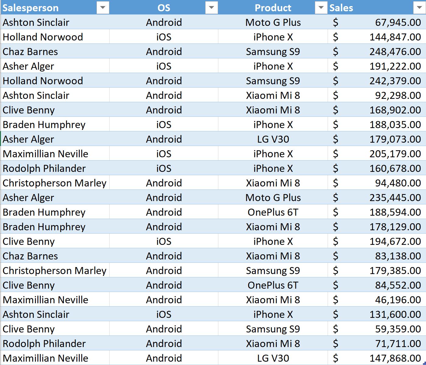
We are going to look at a importing sample data using Power Query, sample data provided by WHO for various countries by regions, depicting data on population, life expectancy, literacy rate, child mortality rate, and so on. Data “WHO.csv” file can be downloaded from here.

Passing Parameters using Manage Parameters

Users can define new parameters by using the “Manage Parameters” dialog in the Query Editor window. Follow the example step by step to understand more about Parameters.

Step 1

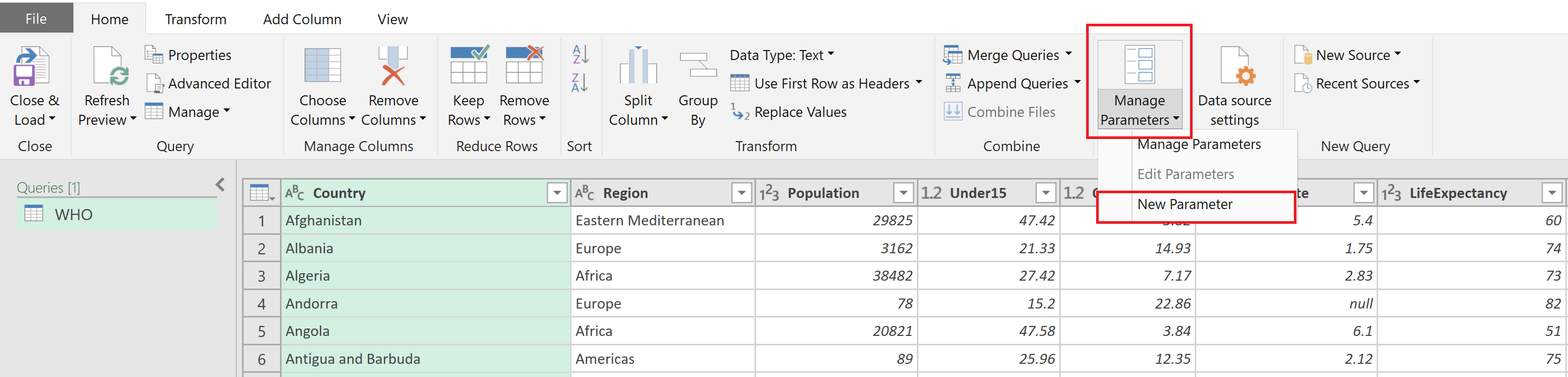
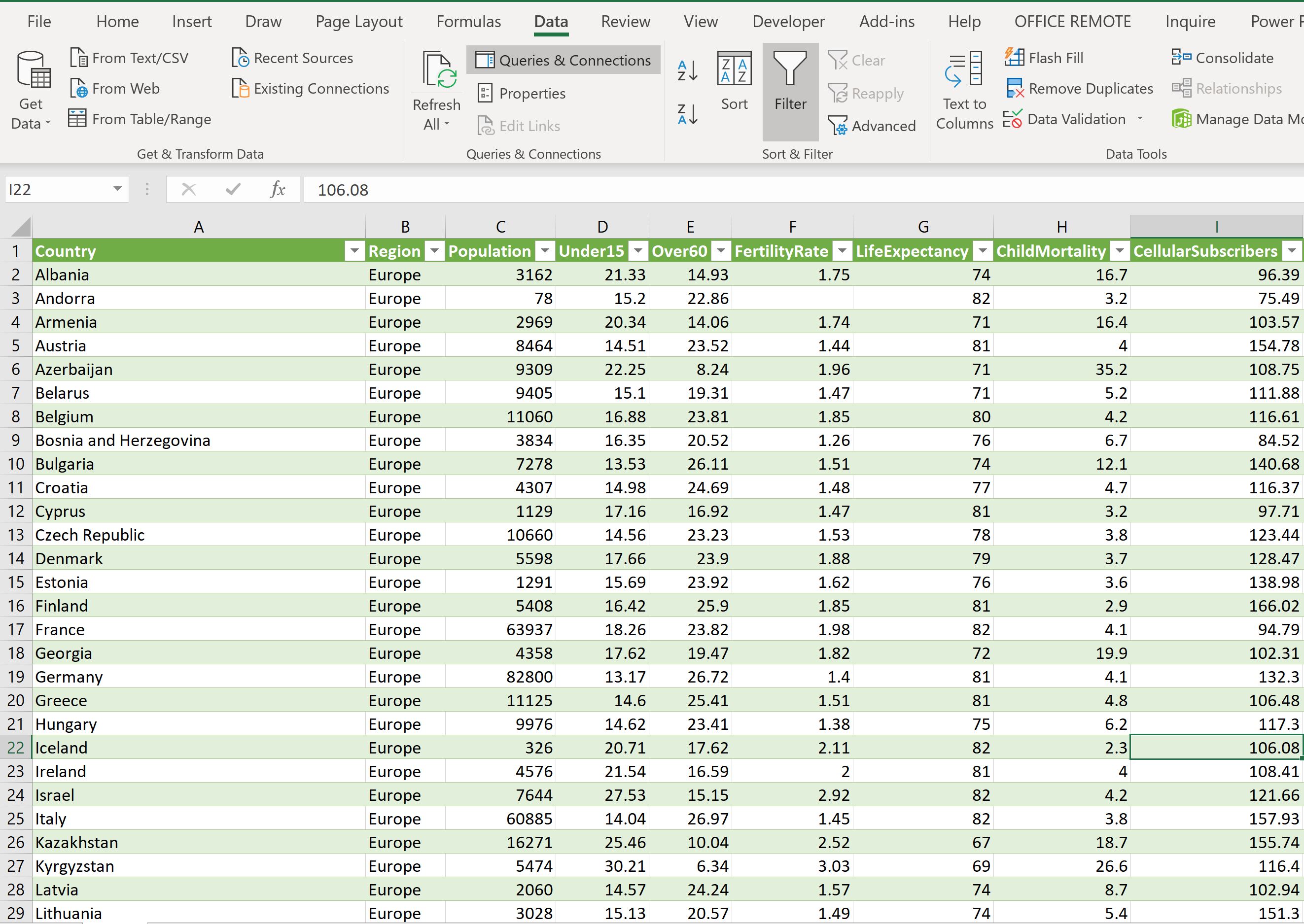
In a new workbook, go to the Data tab, and choose “From Text/CSV” option in the Get & Transform Data section in the ribbon, to import the WHO data using Power Query, and stay in EDIT mode.
In the Home tab, Choose “Manage Parameters” option, and within that select “New Parameter”

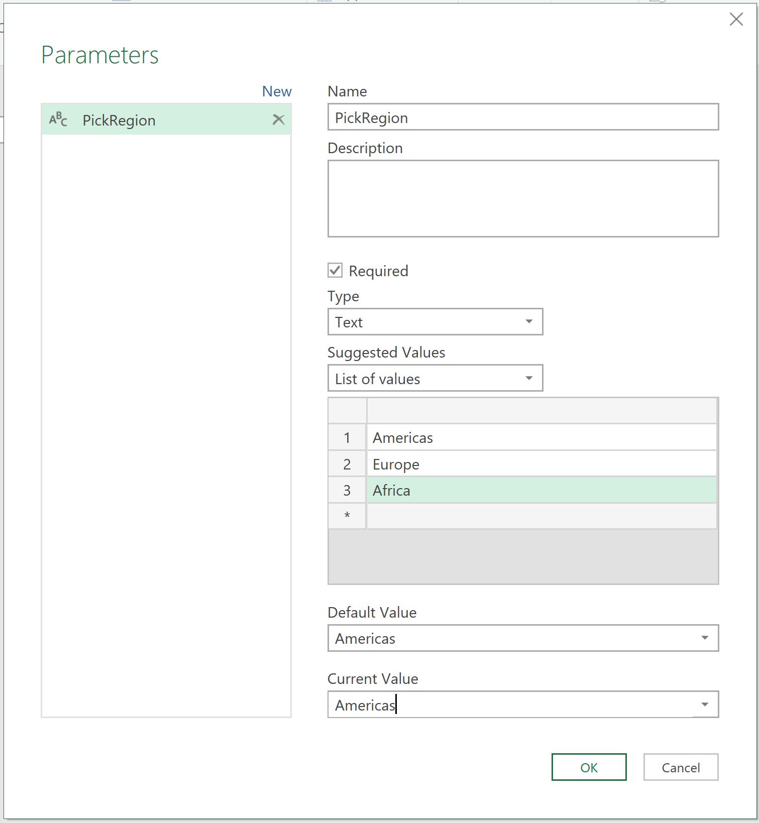
Enter the following details on the Parameter dialog screen.

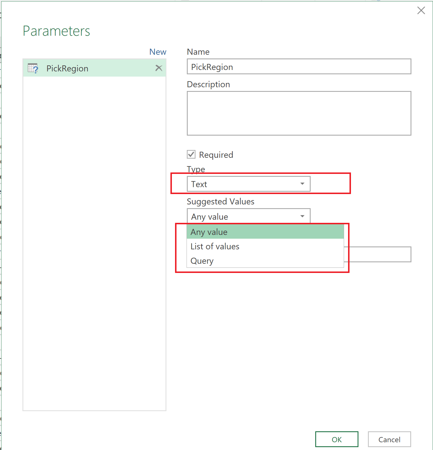
Parameter Name: Put any name you want. In this example, I am putting “PickRegion”.
Parameter Description: Optional, but useful to better understand the purpose and semantics of this parameter.
Optional vs. Required: Specify whether you want to keep the Parameter a required field or not.
Parameter Type: This is the Data Type. Users can define a parameter of type Text, or Date/Time or Decimal Number or True or False, for example. Data type of “Any” provides for more flexibility.
Suggested Values: There are three options available here. Any Type, List of Values and Query. For now, Choose “Any Type”.

Any Type – will allow user to put in any type of value, when specifying the parameter. This allows values to be inputted dynamically. May also be prone to errors.
List of Values – a static list of Accepted Values can be inputted, so users may pick and choose from the list created beforehand.
Query – This would enable dynamic sets of options to be displayed to the user, based on the result of a query.

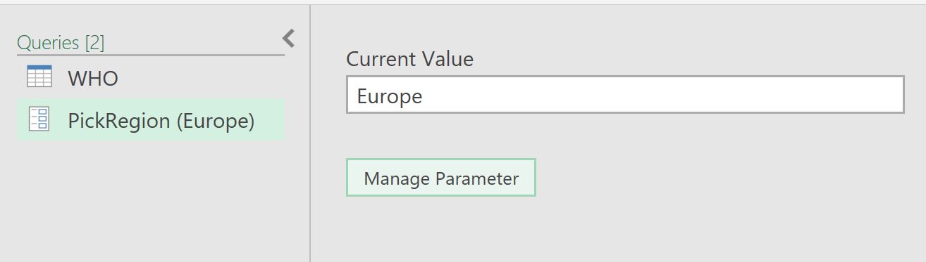
Current Value: Specify any value you want to provide as Current Value. If you keep this blank, it will throw an error. I have specified “Europe”.

You will see that the Parameter is created, and a parameter frame is displayed on screen as such.

Step 2

In this step, we will use the Parameter created in step 1 as a Filter value for the Query.

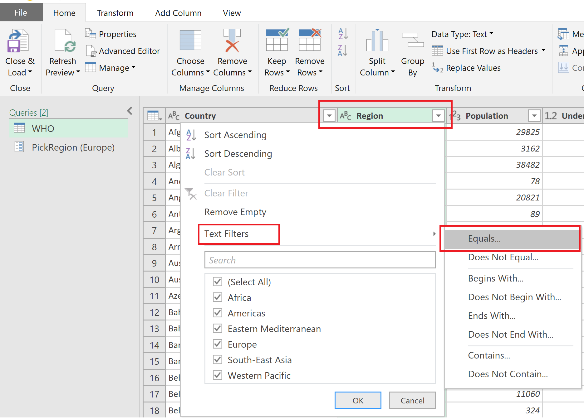
On the dataset of the WHO Query, Filter on the column “Region” as shown below.

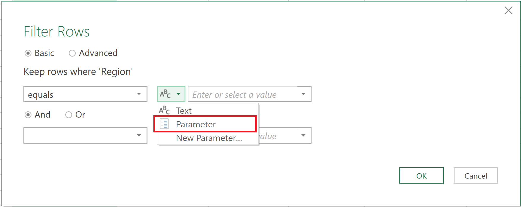
In the Filter Rows dialog box, Select Parameter as the Type of Filter in the icon, and it will default to “PickRegion” as this is the only parameter we have created so far. Hit OK

What this will do, is this will extract the data set based on “Europe” which was the region we had selected as Current Value.

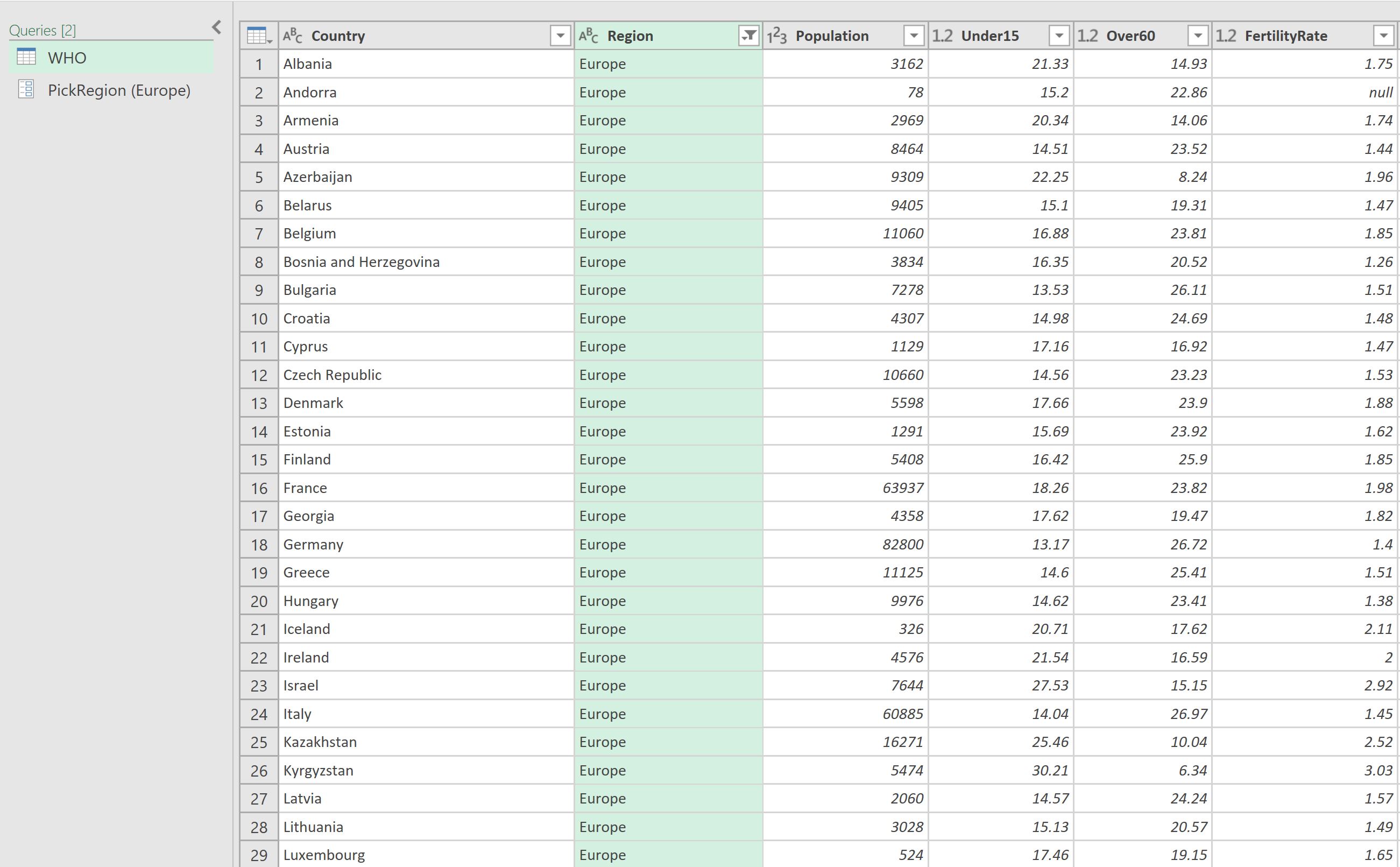
You can choose Close and Load on the Home tab, to load the extract of data into Excel.

Step 3

This time, go back to Power Query, and change the Parameter Suggested Value to “List of Values” instead of “Any Type”.

When you change the value type to List of Values, you will also need to provide all the values you need to show up statically.
Also provide a Default Value and Current Value, and Hit OK.
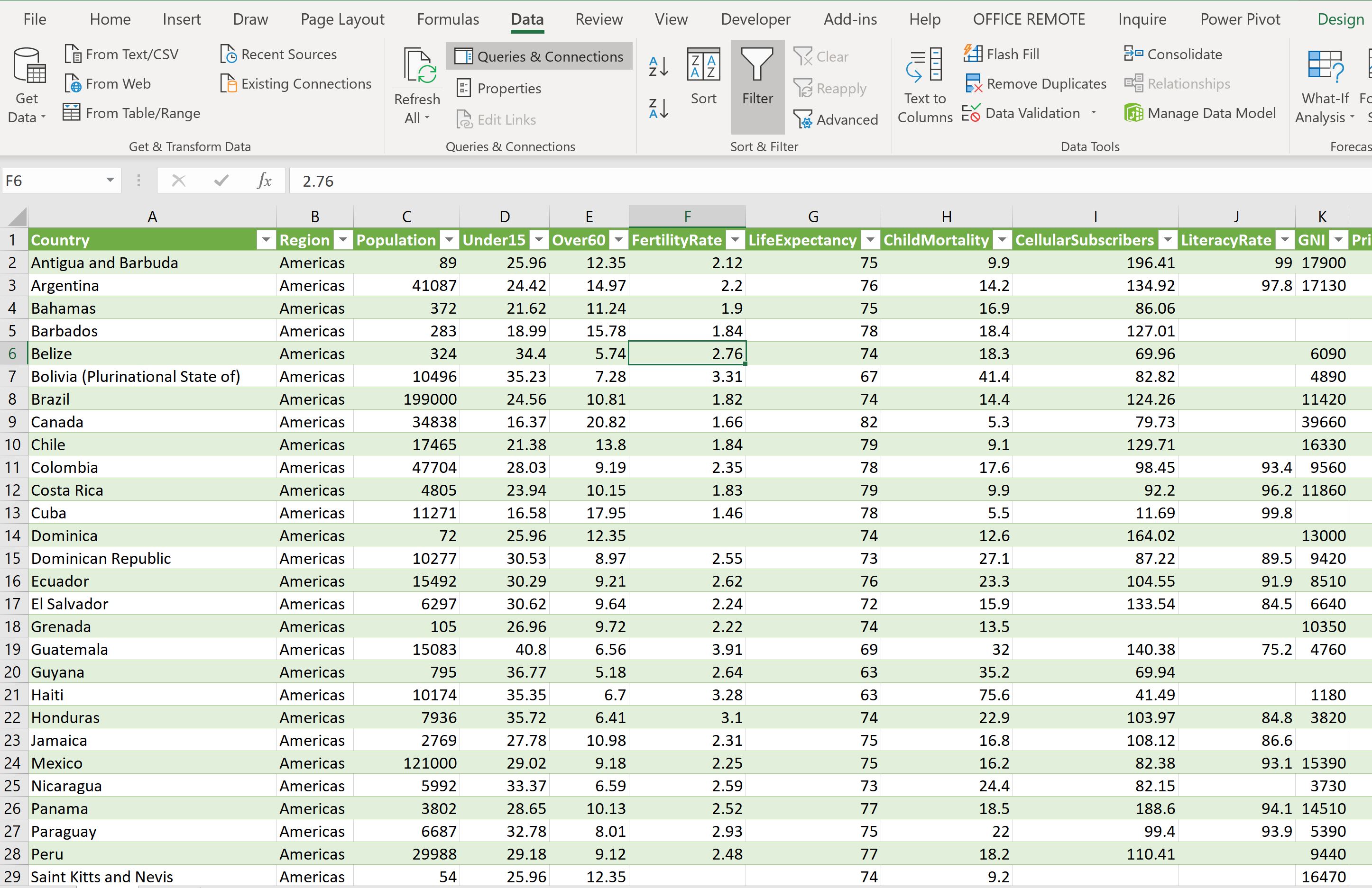
Observe the data set change based on the selection you just gave, in my example, it was Americas. You can choose Close and Load on the Home tab, to refresh your extract of data into Excel based on new selection.

Passing Parameters using a Function

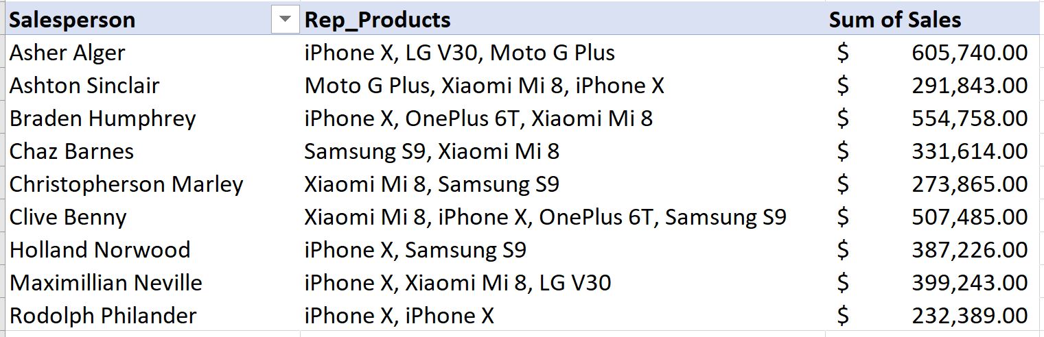
Strategy used in this method is going to be creating a data set using a Power Query, then editing that query to allow a parameter value making it into a function, and then, finally invoking that function in another query that will pass the value to the argument.

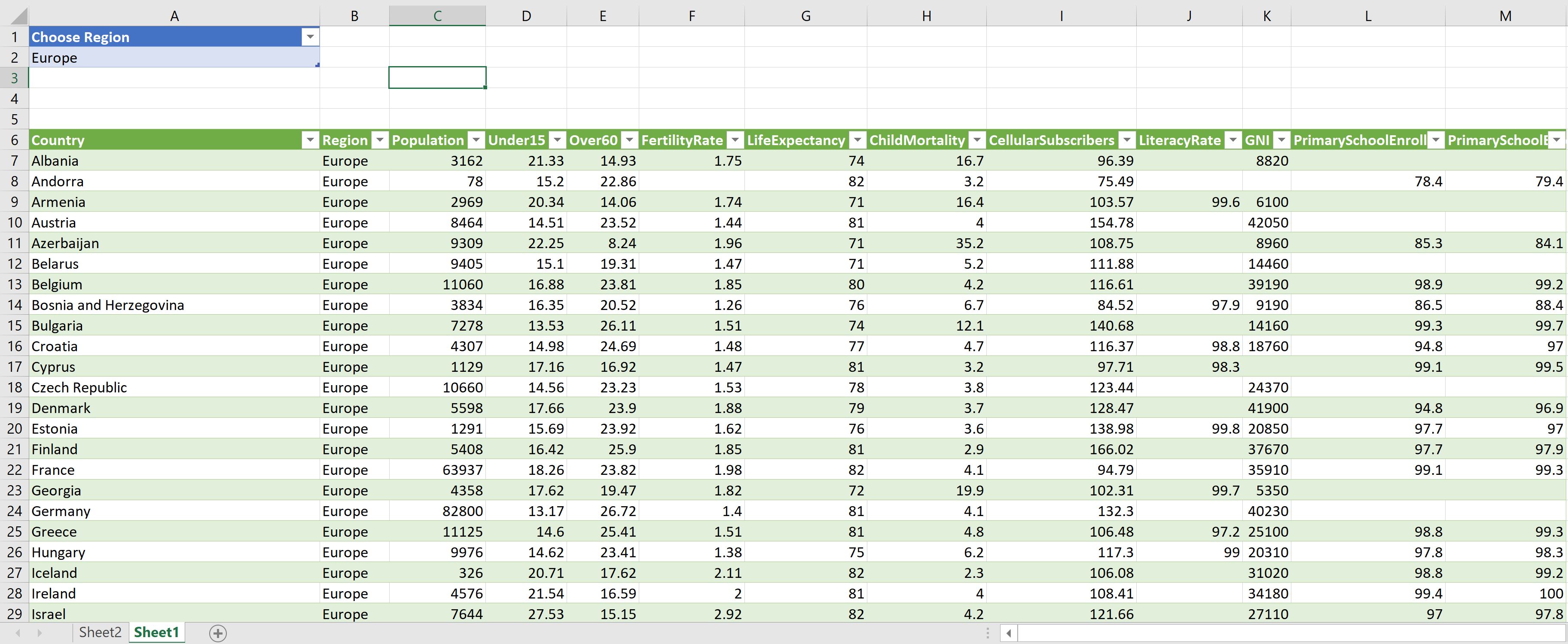
What we want to achieve is, to have a top section where user will have a choice to select a Region (this will be the value passed onto the parameter Function, based on which the WHO data in the lower section is reflected or extracted. See screenshot below:

Top section used to select parameter value, the lower section reflects data based on selection.

Step 1

In a new workbook, go to the Data tab, and choose “From Text/CSV” option in the Get & Transform Data section in the ribbon, to import the WHO data using Power Query, and stay in EDIT mode.

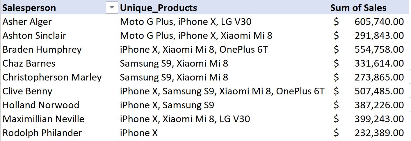
We will rename the Query and “Distinct_Regions”, and perform the following steps:

Select the Column “Region”, and on the ribbon in Home tab, click on “Remove Columns” and “Remove Other Columns”. You will end up with a single column table with the Regions for each row listed.
Now, on the ribbon in Home tab, click on “Remove Rows” and then choose “Remove Duplicates”.

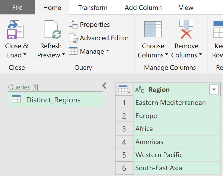
Click on Close and Load, to bring the distinct regions list over to Excel from Power Query.
This table will be used a create a list to be used for Data Validation, which we will need for Parameter section.

Data Validation List created from unique list of Regions

Step 2

In a same workbook, go to the Data tab, and repeat the above step. Choose “From Text/CSV” option in the Get & Transform Data section in the ribbon, to import the WHO data using Power Query, and stay in EDIT mode.

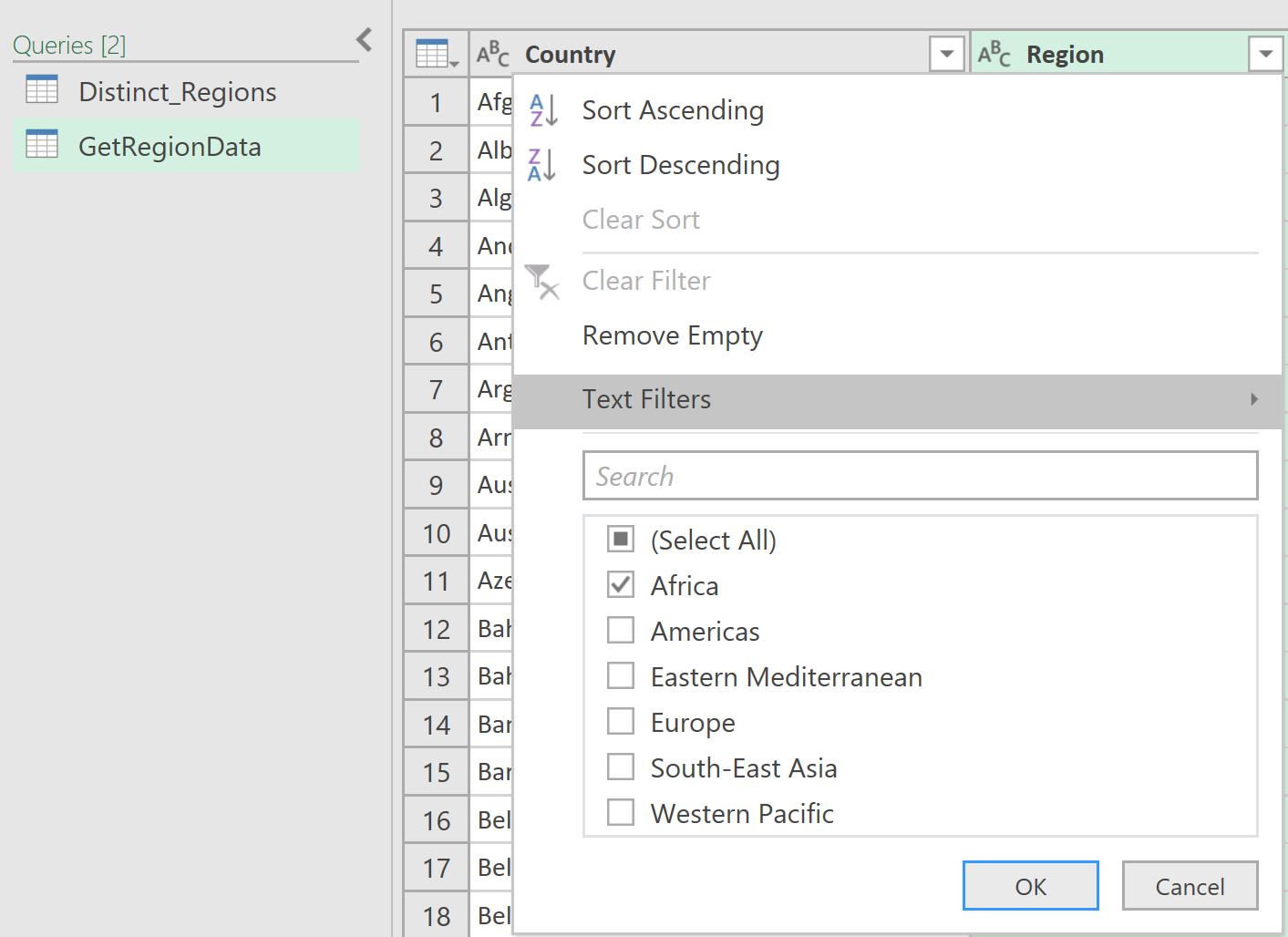
This time, we will rename the Query as “GetRegionData”, and perform the following steps:
Filter on the Region Column, and select any of the Value in the List, for example “Africa” as shown below, and hit OK.

Filter on Region Column for GetRegionData.

Right Click on the Query name “GetRegionData”, and click “Advanced Editor” option. You will see the Formula that has been entered by Excel in M Language.

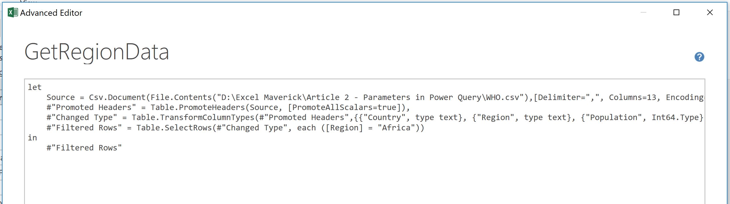
Now edit the code as shown below.

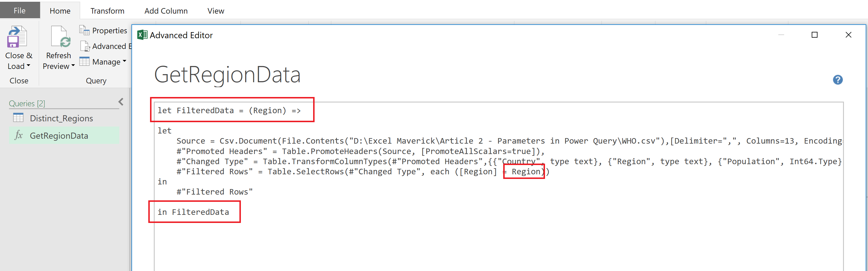
What we have essentially done above, is created a function that uses a parameter “Region”, and this argument is then passed on to the line of code where data gets filtered. We have replaced a static Filter Value “Africa” to a dynamic Filter argument called Region.

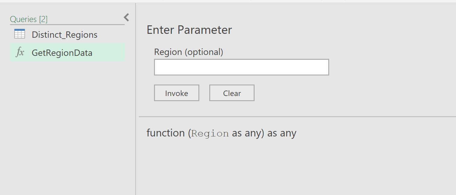
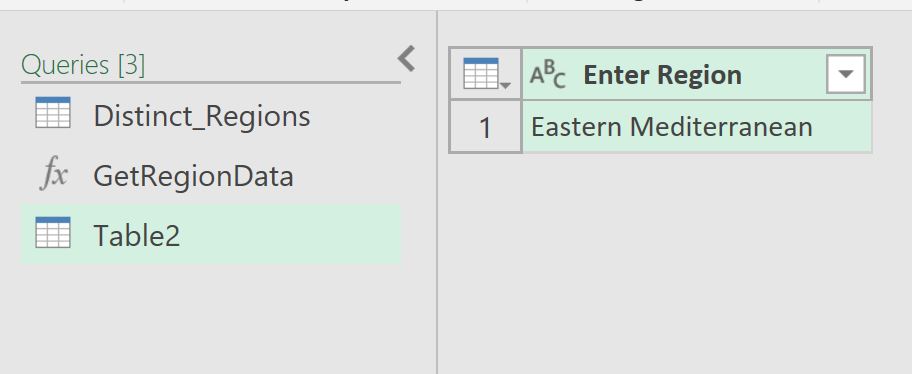
Once done, you will see the Enter Parameter screen as shown below.

Step 3

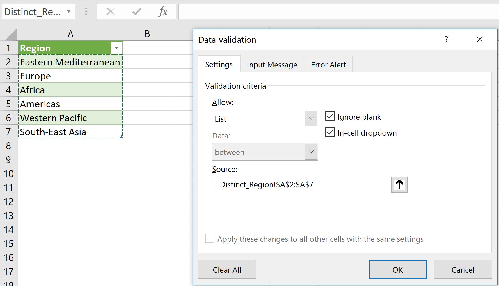
In the Excel, in a new worksheet, in cell A1, enter value “Enter Region”, and in Cell A2, create a Data Validation list based on Regions list in Step 1.

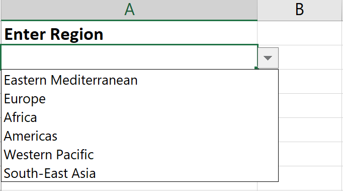
Create a place where user can select value

User will be expected to choose the Value in Cell A2, which will be used as parameter value that the Function will read.

Step 4

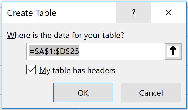
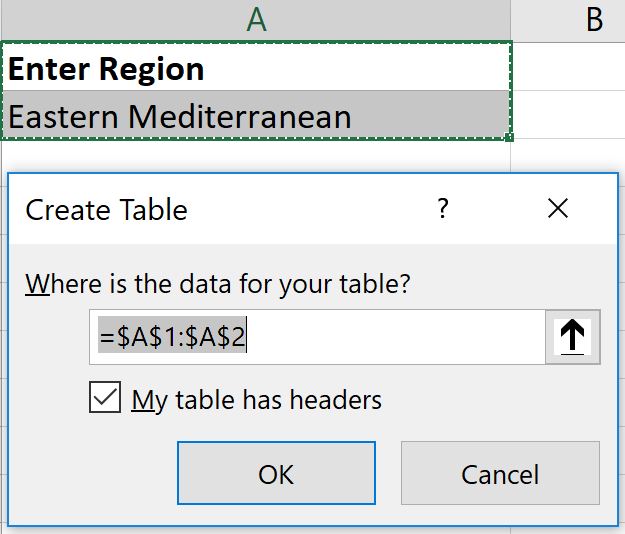
On the same worksheet, on the Data tab, choose “From Table/Range” option, which will bring up a Create Table dialog box. Ensure “My data has headers” option is checked, and hit OK.

Create Table, for the parameter region we just created

The new table will show up in Power Query editor as below.

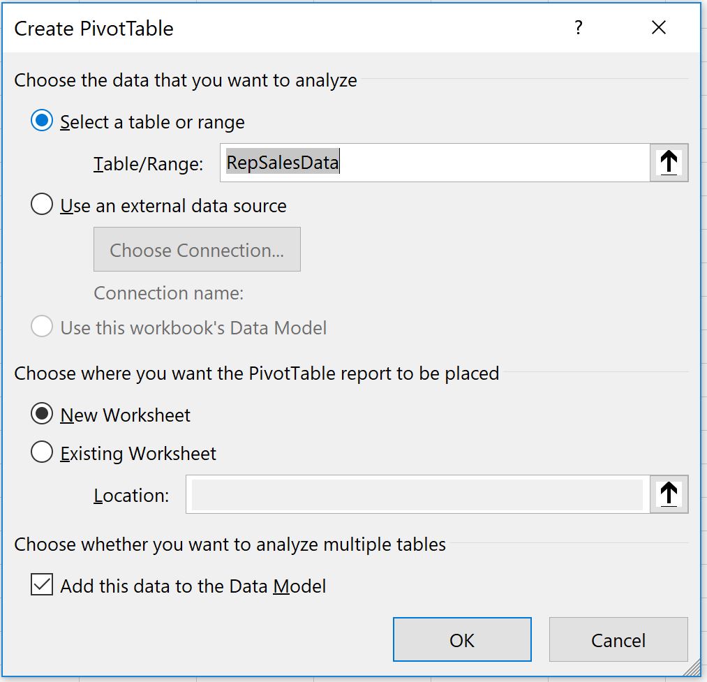
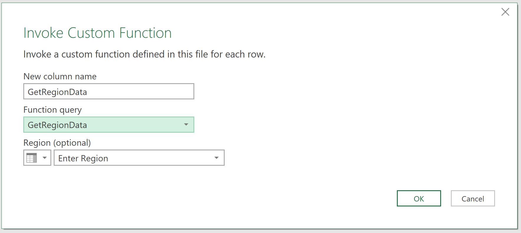
Click on the Table, and on Add Column tab, Click on Invoke Custom Function option. Enter the values in the Function Query field, and hit OK.

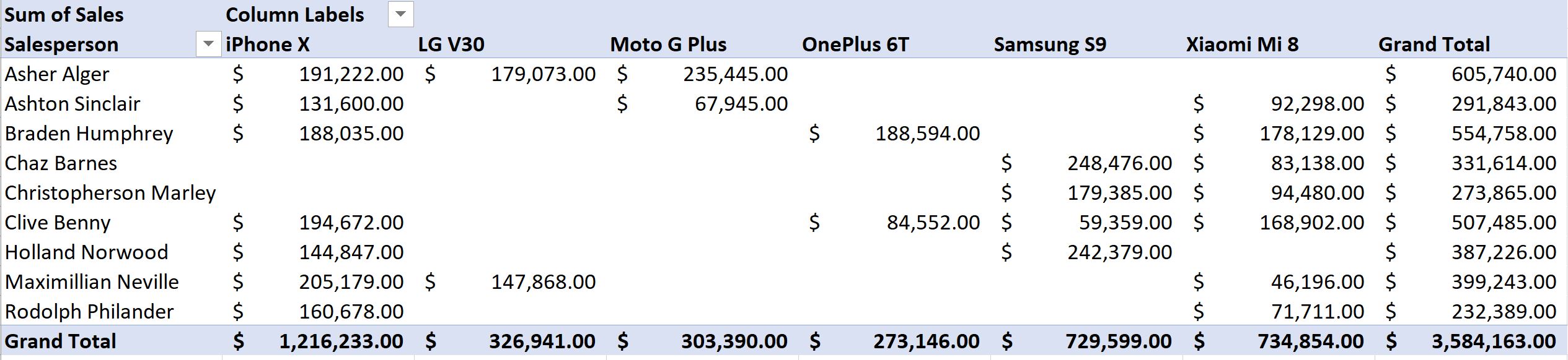
When you have Invokes the Custom Function, this will bring the Filtered Data against the Region selected, as shown below.

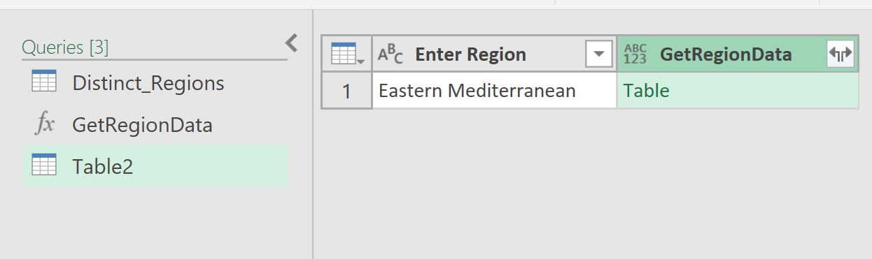
Click on the hyper link Table, which will then list down the data set for that region. Click Close and Load, which will bring the data set into Excel.

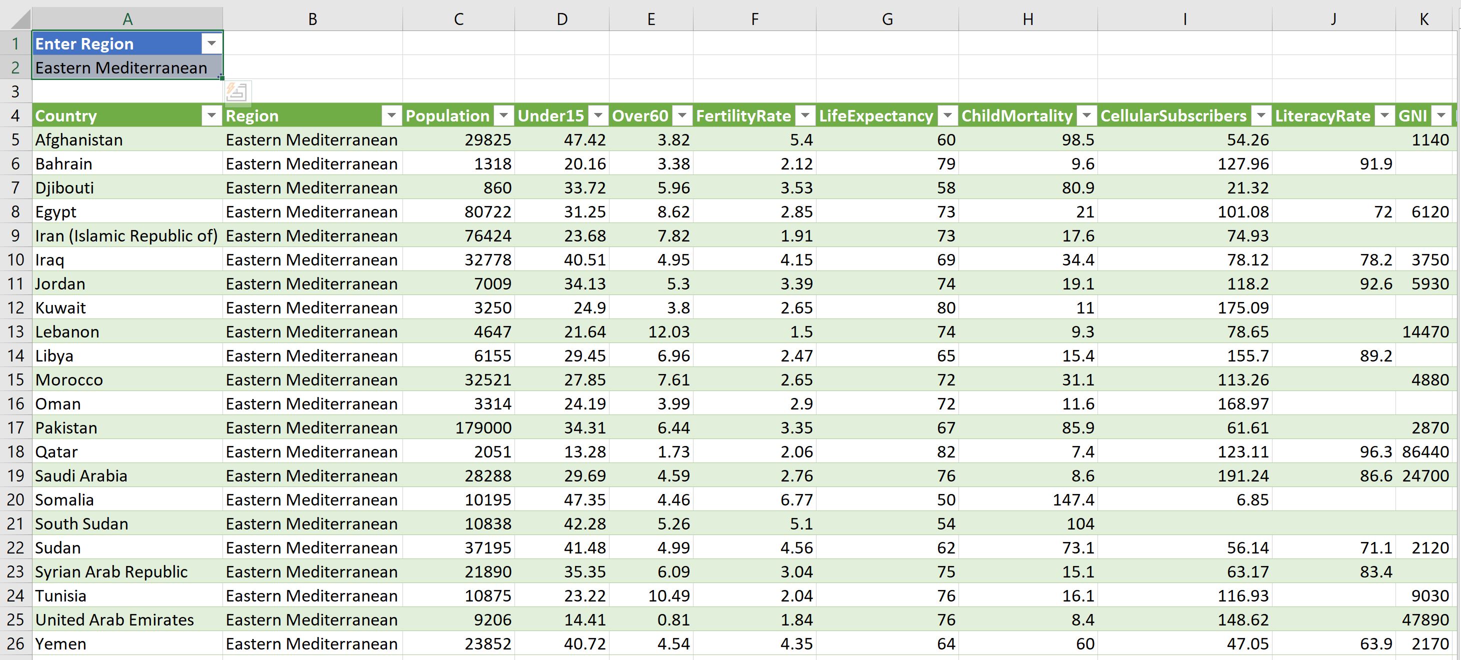
The data is available as we wanted to achieve. In order to test whether the data set changes based on the Region selected, In cell A2, change the selection of region, and hit “Refresh All” option in the data tab. You will see the data set changes based on selection.

Personal word

This is probably the simplest of examples depicted where a parameter table is created that slows for a single value selection. Once you get the underlying concept, you can let your imagination go wild with other fantastic possibilities you could ever dream about.

The example file can be downloaded from this link. Happy Learning !! Also don’t forget to visit my Youtube channel for many more video tutorials.

Gone are the days when you could pivot only with numbers!! Yes, with newer functionalities in Excel you can do pivoting with text as well. In this article, we will ponder upon how to make use of Pivot table to display text values. Pivot tables have been excellent, mainly for summarizing numbers. But, when it came to displaying text in the values area of a pivot table, there wasn’t much available until a DAX function was introduced called CONCATENATEX.

The DAX language has provided us with more possibilities than ever before. It allows for calculations that remained previously impossible. Calculated Fields and Measures are the new terminologies that one must get accustomed to when dealing with pivot tables with advanced functionalities.

Who can use whats described here:

Windows users using Excel 2016 or Excel 2010 to 2013 with Power Query add-in installed
Not available for MAC yet.

Lets first study an example, wherein one may need to have a text value show up in pivot area.

Assume a set of sales data by Sales representative and Product as below.

Traditionally, when using Pivot to analyze the data, one could have summarized the above in the following manner:

However, there was no way to include text values within the pivot area, to show up as below:

Adding a Measure that uses CONCATENATEX function is what makes everything possible. This is what we are going to see in what follows.

The syntax for CONCATENATEX is (Table Name, Expression, Delimiter)

What becomes obvious from the above, is that, it is necessary to create a pivot table based on a source table, and not a range of cells. Next, Expression refers to the Column in the Table whose text values we intend to bring into the pivot area. Lastly, Delimiter is what separates the text values, be it a dash, comma, or a hyphen.

Follow the below steps in sequence to achieve the result of having Text values in Pivot area.

Step 1

Create a Table from the data set. Download the file with the dataset for ready reference. Place your cursor on any one cell in your data set, and then Go to Insert Tab, and choose “Table”. It will bring up a “Create Table” dialog. Select option “My table has headers”, and hit OK. By default, the table will be called Table1. Click on the Table Tools Design tab in the Ribbon and assign a new name for the table as “RepSalesData”.

Step 2

Go to Insert Tab, and choose “PivotTable”. This will bring up a dialog box “Create PivotTable”. Ensure Table/Range field shows up as “RepSalesData”. Choose “New Worksheet”, and most importantly, check the option “Add this data to the Data Model”, and hit OK.

Step 3

This will show up the Pivot Table Fields section on the right side of the screen. When your pivot table is based on the Data Model, you will see a difference in the Pivot Table Fields list. The name of the table will appear at the top of the fields from that table. Right-click on the name of the table “RepSalesData” and choose Add Measure.

Pivot Table Fields, Table shows up at the top of the Field list

Step 4

You will get a new dialog screen “Measure” where the magic begins. Give a Measure name “Rep_Products”, and description. In the formula area, enter the below formula:

=CONCATENATEX(RepSalesData,RepSalesData[Product],”, “)

Click on “Check DAX Formula” button. This will check for error in the formula entered. If there are no errors, it will display so. Choose “General” as the category for the Measure newly created. Note, for a text result, the only valid choice is General, so leave the selection as General. Hit OK to create the new Measure.

Measure is defined, Category chosen as General

Step 5

The new measure will not show up in the pivot table, instead it will show up as a new field in the Pivot Table Fields list. Start to build your pivot table by dragging fields to the Rows and Columns area. Drag the new field to the Values area. On the PowerPivot Tools Table Design Tab, turn off the Grand Totals for both Rows and Columns.

Step 6

Finally, you will see the Product list showing up next to each other in the “Rep_Products” column in the Pivot table.

Product List showing as Text values in Pivot area

However, if you observe closely, the last row in the pivot table shows up with iPhone X repeated twice. What this means is that the Sales representative has sold iPhone X twice in the given data set. If your intention is to only display the unique products sold by that Sales rep, you need to nest the VALUES function within CONCATENATEX function.

Step 7

Edit the measure we created above, and replace the below formula in lieu of the earlier one.

=CONCATENATEX(VALUES(RepSalesData[Product]),RepSalesData[Product],”, “)

With the VALUES function, duplicate values are removed, and only unique values are returned.

Unique Product List showing up as Text Values in Pivot area

Will also be updating my YouTube Channel with a tutorial video of the above example, and how to get the text value show up in Pivot. Keep watching, and send me comments.

Category: Power Query

Passing parameters to queries in Power Query

Passing Parameters using Manage Parameters

Passing Parameters using a Function

Personal word

Pivot with Text