
Gone are the days when you could pivot only with numbers!! Yes, with newer functionalities in Excel you can do pivoting with text as well. In this article, we will ponder upon how to make use of Pivot table to display text values. Pivot tables have been excellent, mainly for summarizing numbers. But, when it came to displaying text in the values area of a pivot table, there wasn’t much available until a DAX function was introduced called CONCATENATEX.
The DAX language has provided us with more possibilities than ever before. It allows for calculations that remained previously impossible. Calculated Fields and Measures are the new terminologies that one must get accustomed to when dealing with pivot tables with advanced functionalities.
Who can use whats described here:
- Windows users using Excel 2016 or Excel 2010 to 2013 with Power Query add-in installed
- Not available for MAC yet.
Lets first study an example, wherein one may need to have a text value show up in pivot area.
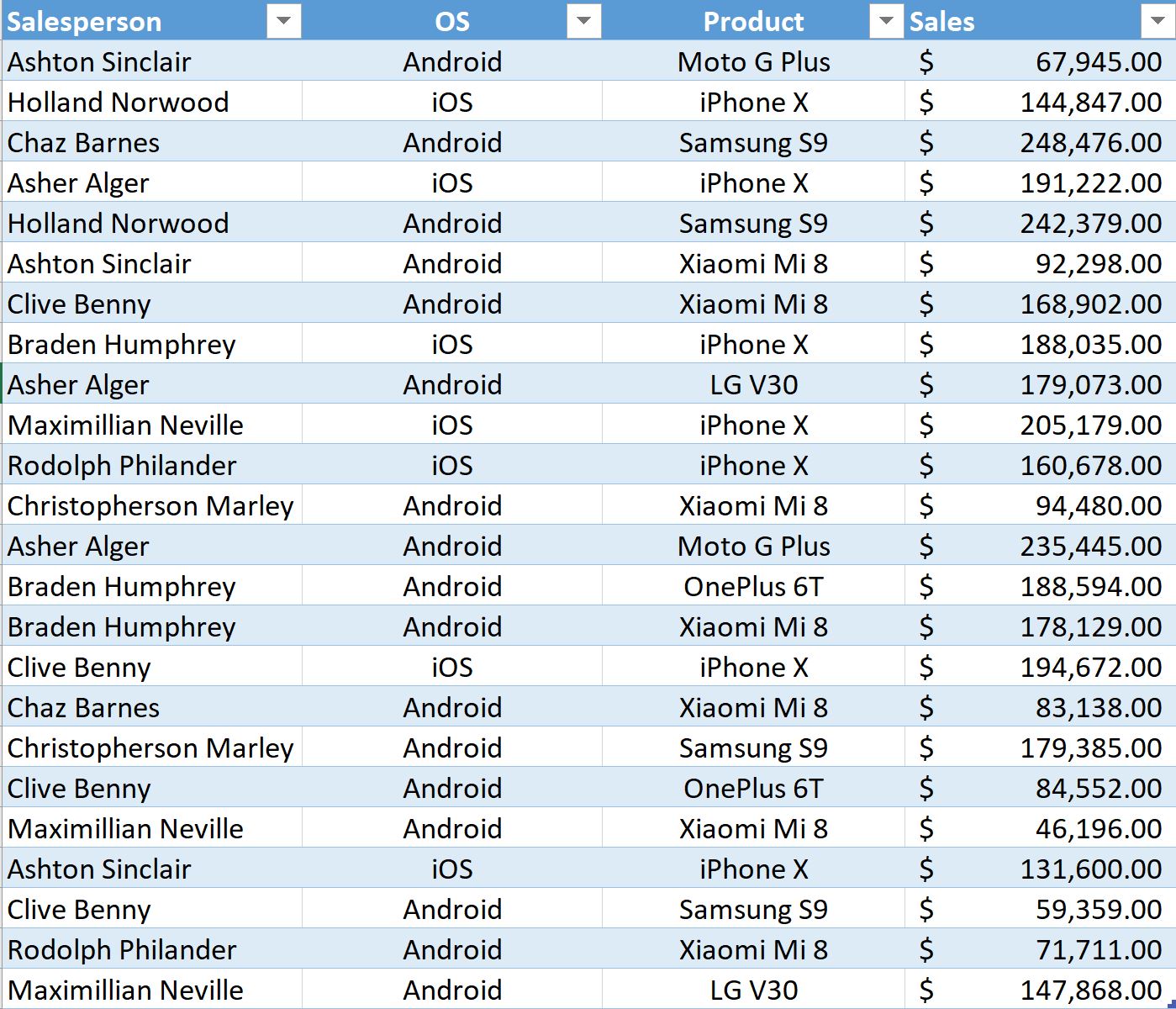
Assume a set of sales data by Sales representative and Product as below.
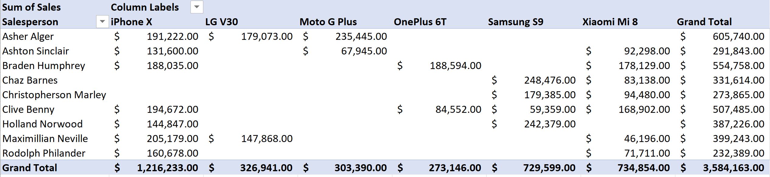
Traditionally, when using Pivot to analyze the data, one could have summarized the above in the following manner:
However, there was no way to include text values within the pivot area, to show up as below:

Adding a Measure that uses CONCATENATEX function is what makes everything possible. This is what we are going to see in what follows.
The syntax for CONCATENATEX is (Table Name, Expression, Delimiter)
What becomes obvious from the above, is that, it is necessary to create a pivot table based on a source table, and not a range of cells. Next, Expression refers to the Column in the Table whose text values we intend to bring into the pivot area. Lastly, Delimiter is what separates the text values, be it a dash, comma, or a hyphen.
Follow the below steps in sequence to achieve the result of having Text values in Pivot area.
Step 1
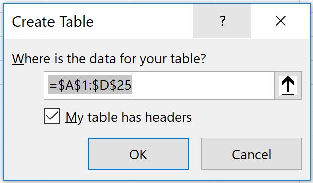
Create a Table from the data set. Download the file with the dataset for ready reference. Place your cursor on any one cell in your data set, and then Go to Insert Tab, and choose “Table”. It will bring up a “Create Table” dialog. Select option “My table has headers”, and hit OK. By default, the table will be called Table1. Click on the Table Tools Design tab in the Ribbon and assign a new name for the table as “RepSalesData”.
Step 2
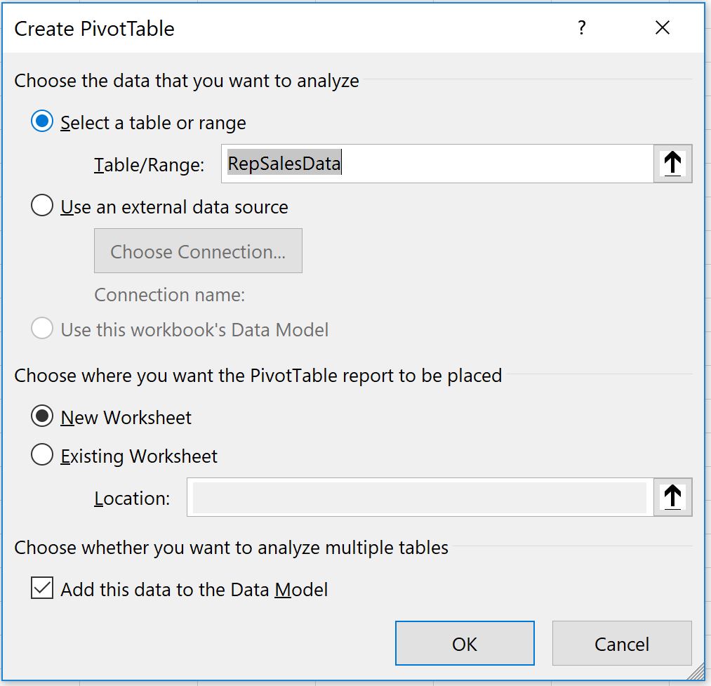
Go to Insert Tab, and choose “PivotTable”. This will bring up a dialog box “Create PivotTable”. Ensure Table/Range field shows up as “RepSalesData”. Choose “New Worksheet”, and most importantly, check the option “Add this data to the Data Model”, and hit OK.
Step 3
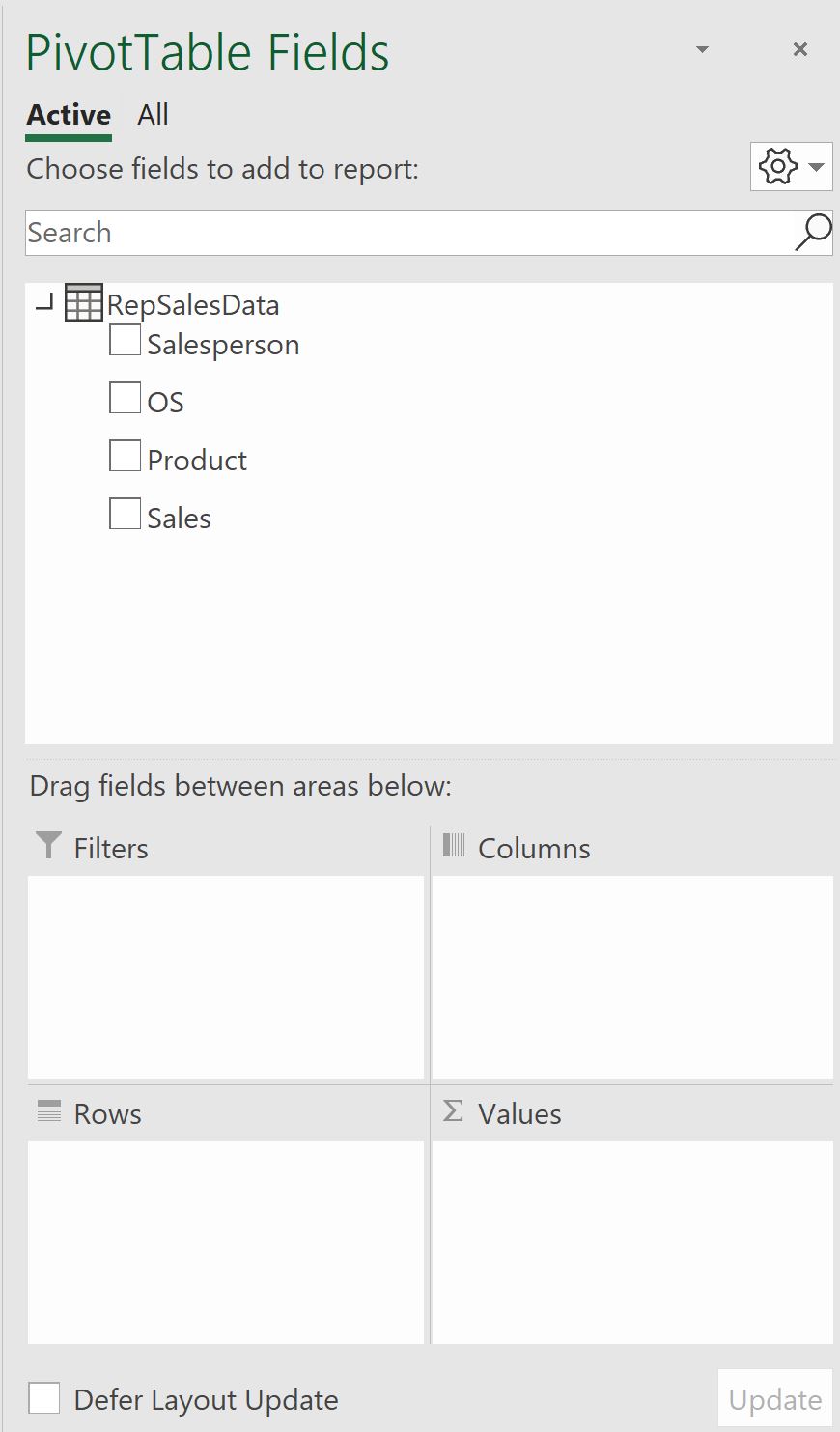
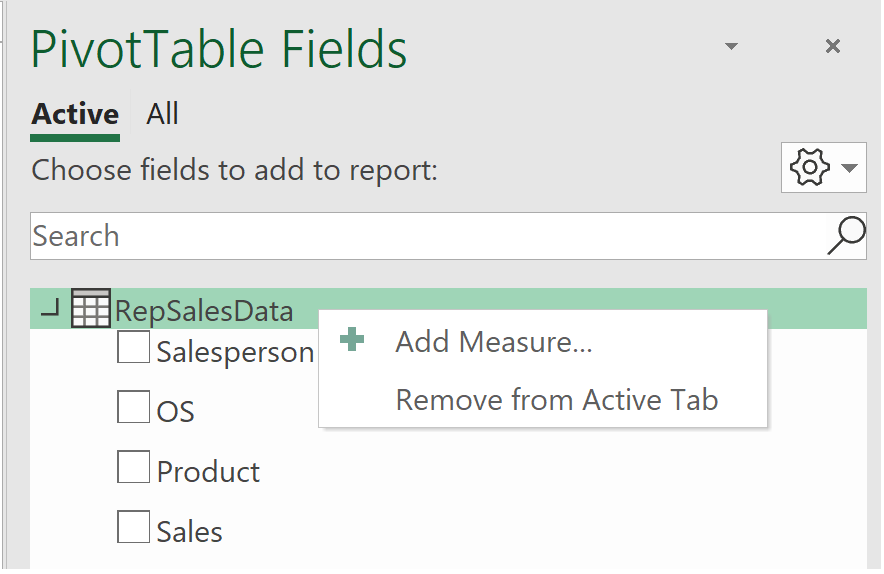
This will show up the Pivot Table Fields section on the right side of the screen. When your pivot table is based on the Data Model, you will see a difference in the Pivot Table Fields list. The name of the table will appear at the top of the fields from that table. Right-click on the name of the table “RepSalesData” and choose Add Measure.
Step 4
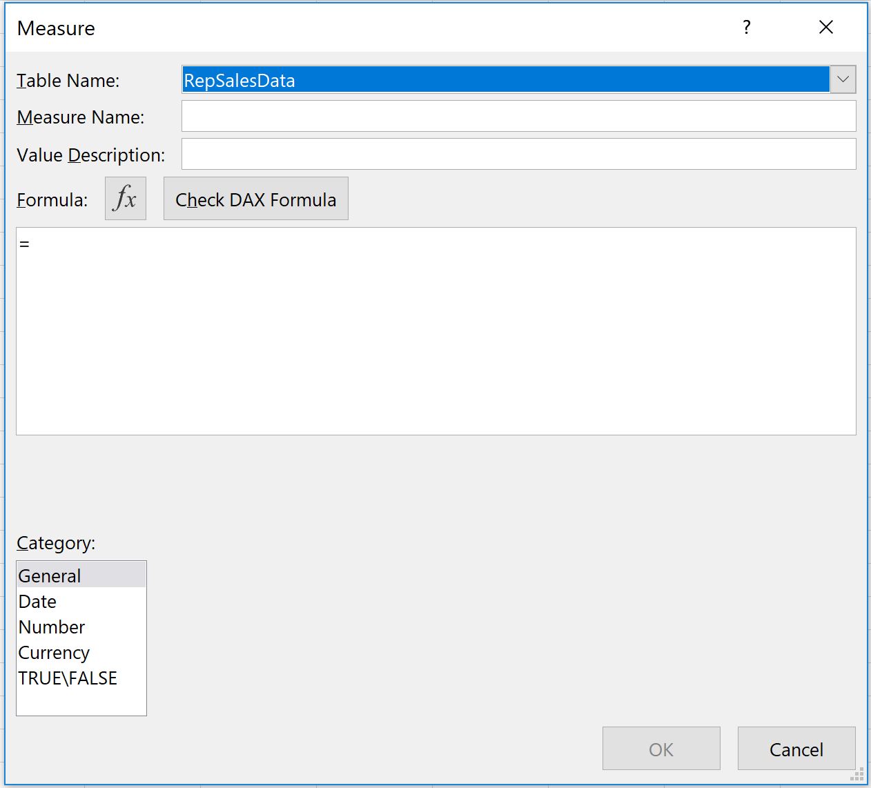
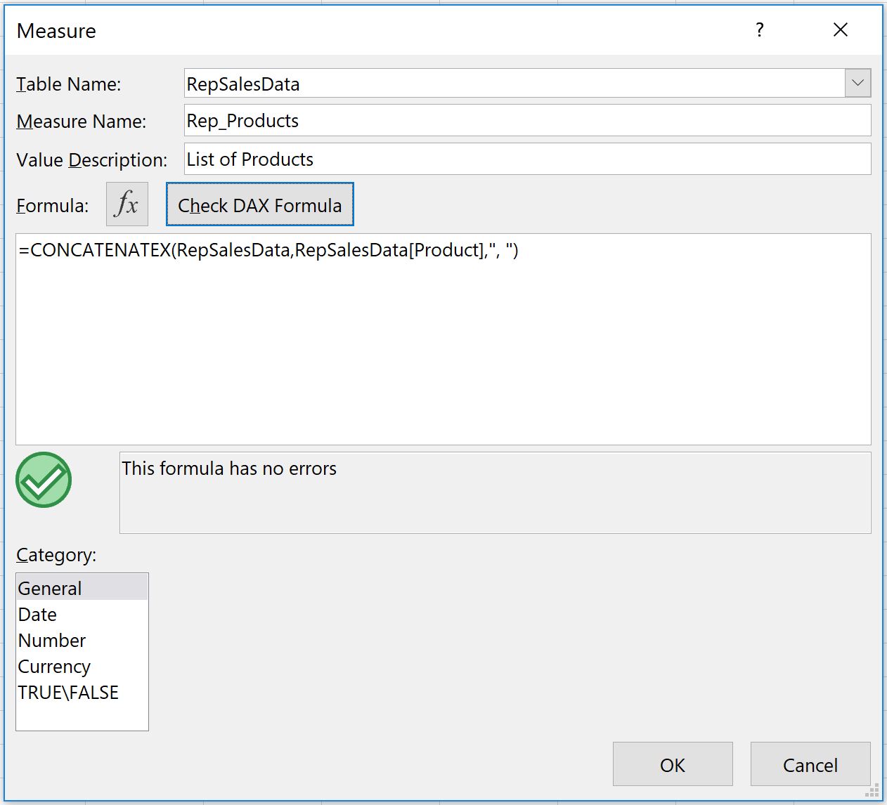
You will get a new dialog screen “Measure” where the magic begins. Give a Measure name “Rep_Products”, and description. In the formula area, enter the below formula:
=CONCATENATEX(RepSalesData,RepSalesData[Product],”, “)
Click on “Check DAX Formula” button. This will check for error in the formula entered. If there are no errors, it will display so. Choose “General” as the category for the Measure newly created. Note, for a text result, the only valid choice is General, so leave the selection as General. Hit OK to create the new Measure.
Step 5
The new measure will not show up in the pivot table, instead it will show up as a new field in the Pivot Table Fields list. Start to build your pivot table by dragging fields to the Rows and Columns area. Drag the new field to the Values area. On the PowerPivot Tools Table Design Tab, turn off the Grand Totals for both Rows and Columns.
Step 6
Finally, you will see the Product list showing up next to each other in the “Rep_Products” column in the Pivot table.
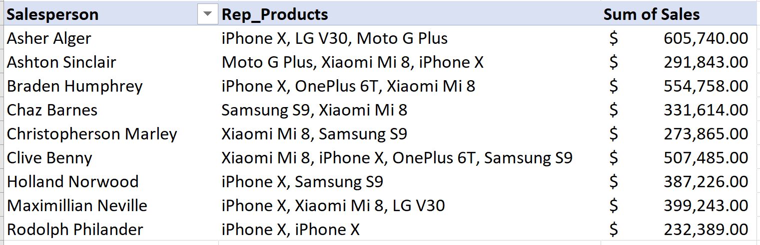
However, if you observe closely, the last row in the pivot table shows up with iPhone X repeated twice. What this means is that the Sales representative has sold iPhone X twice in the given data set. If your intention is to only display the unique products sold by that Sales rep, you need to nest the VALUES function within CONCATENATEX function.
Step 7
Edit the measure we created above, and replace the below formula in lieu of the earlier one.
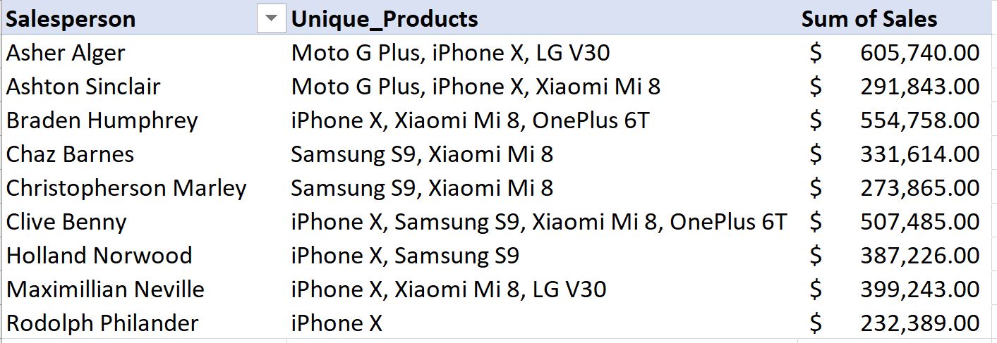
=CONCATENATEX(VALUES(RepSalesData[Product]),RepSalesData[Product],”, “)
With the VALUES function, duplicate values are removed, and only unique values are returned.
Will also be updating my YouTube Channel with a tutorial video of the above example, and how to get the text value show up in Pivot. Keep watching, and send me comments.